Problem Definition
Project Overview
The price of financial assets that are traded on public markets is established by supply and demand. Under the efficient market hypothesis, all available information about the underlying asset/company should be always completely and fully included in the price. But at times this is not the case because there can be different interpretations of and opinions on fundamental information may vary, and investors may get too fearful or too excited about a stock. The longer-term view of a share price is normally in line with the fundamentals of the company - eg. Profits & Losses, the health of the Balance Sheet, and its position in the competitive landscape it operates in. On shorter time scales (seconds, hours, days, and even weeks), investors may not have fully built all available information into a rational valuation of a share. In those moments, fear or a short term scandal might drive share prices irrationally low, or a bubble mania might overinflate prices as late investors rush in buying, driving prices ever higher.
While fundamental investment analysis deals with the former, technical analysis attempts to identify patterns in the historic and recent stock prices to predict future prices. Investment strategies based on technical analysis aim at generating investment returns by capitalizing on the identified patterns. A very simple classic trading strategy built on technical indicators is to look at if the stock price is above a moving average and to consider that an uptrend during which the stock should be owned until the stock price drops below the moving average (signaling a downtrend).
This project will explore how to use machine learning to predict trading signals based on technical analysis. The implementation will be in Python using sci-kit learn and free historical stock data. One specific trading strategy will be evaluated and the predicted trading signals will be backtested to find out how much better or worse an investor would have performed compared to simply buying the stock and holding it for the observation period (Buy and Hold Strategy).
We will be using a small subset of stock data from Quandl's extensive database of historical daily stock prices. The (very aspirational) goal is to outperform the stock market. To no surprise, our model fails to produce a guaranteed way to quick wealth but along the way, we will tackle some interesting data processing challenges, build a few models, and figure out how to backtest the performance. We will also have built a solid foundation for future explorations with other models and trading strategies.
Problem Statement
The goal is to predict profitable trades for one specific trading strategy:
-
- On day N,
- based on daily High, Low, Open, and Close data and Trading volume, and
- a few generated technical indicators (we will implement Relative Strength Index - RSI and Simple Moving Averages - SMA), and
- a few additional features (such as "50 day SMA crossed above 200 day SMA" and "Close price is below 200 day SMA"and "RSI was above 80"),
- decide if a stock should be purchased on the next day at the opening price (Market Order on the Open on day N+1)
- for a holding period of 10 days (sell on the Open with Market Order on day N+10)
- if the expected profit is at least 2.5%.
- We will include n_feature_days of prior data point for the decision on day N.
I.e. if used for real trading, the model would tell us in the evening of day N if we should buy a certain stock the next morning and then sell it another 9 days later (on day N+10) in hopes of making at least 2.5% profit on that trade. The model will make that decision based on prior market data from day N and additional prior days.
There is nothing scientific about the specific parameter chosen, but as we will later see, being able to successfully make all these trades would indeed be a very profitable strategy because it essentially participates in most high-profit days and avoids downtrends in the stock price. And the workflow and model we will develop could very easily be modified for other sets of parameters (different timing and different profit expectation).
Phrased this way, our stock market prediction becomes a Classification problem (should we buy stock X or not?). Since stock prices are time series data, we will need to make sure that we are not using any data from future days past day N (that would probably make our model extremely smart but also completely worthless for real use until we figure out how to time travel).
Along the way, we will need to address the following challenges:
-
- acquire stock market data for a set of ticker symbols
- implement the strategy calculation to see on which days there was a profitable setup for the strategy
- calculate technical indicators and add them to the dataset
- reshape the data into something we can use for machine learning
- train models and optimize their hyperparameters for better prediction results
- build a backtesting mechanism to calculate what profits the trades would generate
- analyze the predicted trading signals with a backtest to see if we should use real money with this algorithm (answer: not quite yet...)
- figure out how we could improve this model going forward
There are several other ways of analyzing time series - notably using LSTM networks or using trend based models (such as ARIMA or specific implementations like Facebook Prophet) - but we will treat this as a classification problem and integrate the unique characteristics of a time series into the model by careful feature generation.
The expected solution is an optimized model that can predict profitable trades.
Success Metrics
The ultimate success metric for the model will be if the predicted trades generate profits. As a first goal, the trades should not lead to losses, and second, they should perform better than a buy-and-hold strategy where we just buy the stock on the first day of the evaluation period and not sell it until the last day of the test period.
Since it is not common to be able to make 2.5% profit in 10 days, we expect our data to imbalanced (we will have less than half days with a trade signal). One strategy to handle imbalanced classes would be to resample but with time series data that might introduce lookahead bias (ie cheating by learning from the future). So we will need to use scoring metrics are more robust for imbalanced data. We will focus on F-scores (see here, here, and here for some discussions on the topic) during model training.
Analysis of input data
Using the Pandas DataReader we can quickly build a function to import daily stock price data that is already adjusted for splits and dividends:
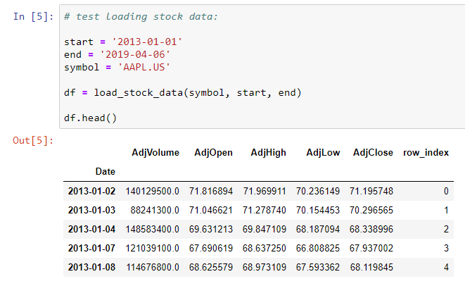
The data is already all numerical and does not contain any null or NaN values so no data cleaning is required. After defining a list of companies we want to train our model on, we can download the data and then build one dataset that contains all prices:
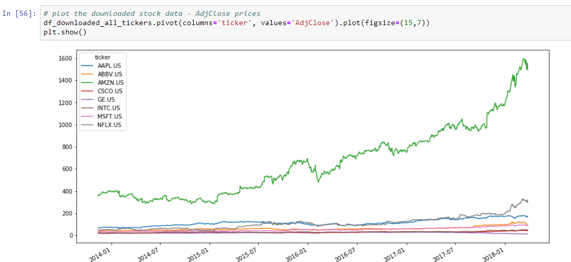
To keep model training manageable, we will limit our data set to only 8 stocks. Increasing this list would certainly enhance the model accuracy but also slow down training more.
Methodology
Data Preprocessing
The data processing step is one of the three key steps in this project (the other two are model training and building a way to calculate and compare the trade performance as a backtest) since our raw data from Quandl needs three types of treatments before we can train our model with it:
-
- calculating the results of the trading strategy - since we currently don't even have a target column without this
- adding additional columns in the form of technical indicators and combinations of those
- reshaping the data since our ML model will need all features to predict the target value in one row - whereas the data from prior days is currently in different rows in the dataset
Calculating the prediction target column - should we buy the stock the next day?
For each row (day) in our data of stock prices, we need to add a flag that tells us if we should buy the stock the next day at the market Open price. We determine this by calculating the profit for "buy tomorrow and sell 9 days later" and then compare it to our profitability threshold of 2.5%:
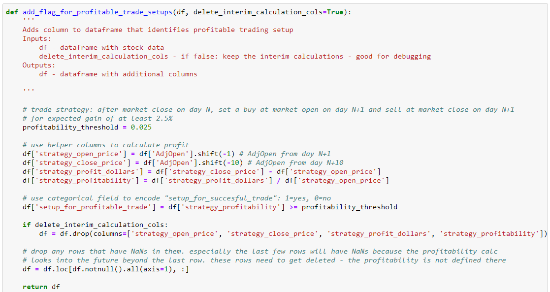
Notice that the profitability is not known for the last 10 days of our original stock data since we don't know yet if the trades would turn out profitable or not. So we will remove those data points from our dataset. We now have a new column that tells us for day N if we should have bought the stock the next day for a profit of 2.5% or more in the next 10 days.
Feature Engineering - Part 1 - adding Technical Indicators
The excellent library TA-LIB provides access to over 150 commonly used technical indicators. We will use append our data with three Simple Moving Averages (SMA) of different lookback lengths (10 days, 50 days, and 200 days; all counted in stock market days - ie rows in our dataframe). SMAs indicate trends and smooth out shorter-term fluctuations. Additionally, we will use the Relative Strenght Indicator (RSI) that indicates extreme and quick price swings (values below 20 can be considered oversold and values over 80 can be considered overbought).
We also combine the stock price data and the SMAs to create second-order features such as "did the stock price today cross over the SMA50" and "ratio of stock close price to SMA 200" and even "is the SMA200 higher than the SMA50". By adding these combinations, we are introducing features that are commonly used in technical analysis to identify changes in trends and market extremes. Many, many more indicators could get added and combined in an attempt to build better prediction accuracy.
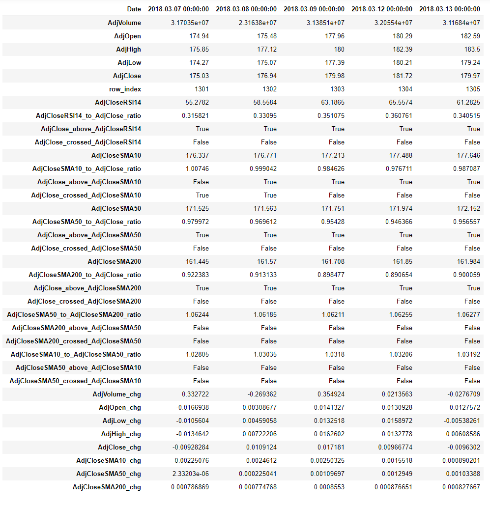
Our enriched data set now has these columns (flipped on the side for easier displaying):
Feature Engineering - Part 2 - Reshaping the data to include the prior day's information in the row for each day
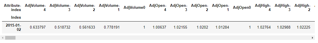
Until now, we have the data for day N in one row but our idea is to use information from prior days when we make a prediction for day N. In order to use a classic Classification model, all data for that prediction needs to be in that row. Therefore, we need to reshape our data and create additional feature columns for the existing ones that contain the feature values for the prior days. We limit ourselves to n_feature_days and unstack the data and then re-assemble a new dataframe. This leads to an increase in features by n_feature_days and makes our dataset richer for each day N. We identify the columns with data from prior dates with a suffix. For example, the column AdjCloseSMA200-4 now contains the value of the 200 day Simple Moving Average of the Adjusted Close price from 4 days ago. Similarly, AdjVolume-2 is the Adjusted Volume from two days prior. The data has also been normalized to the current day to eliminate meaningless absolute values and instead focus on changes:
The current implementation to build this much wider dataframe is computationally expensive as it uses a loop instead of using vectorized computations that would likely improve performance significantly and allow for more experimentation with additional technical indicators and combinations. However, even that faster implementation would still lead to the same number of columns, which ultimately then determine how slow the ML training process will become.
As a small additional step in feature engineering, we also add the month, day, week, and year of the date.
Finally, the data is split into training and test data. Since we need to avoid lookahead bias (ie time travel into the future and using unknown future data), the test set contains the newest data.
Machine Learning Implementation and Refinement
We use a simple RandomForestClassifier with its default parameters to establish a baseline and to confirm that we can process the input data. We then use a GridSearch over a hyperparameter-space, taking care to ensure we use TimeSeriesSplit to prevent lookahead bias in the folds.
As mentioned above, the imbalanced nature of our data lends itself to F-Beta scores, where beta can shift priority between precision and recall. The perfect prediction would avoid false negatives (to avoid missing out on profitable trades) and avoid false positives (to avoid unprofitable trades). GridSearches were performed with beta = 0.5, 1.0, and 2.0 and model predictions for the best models were saved.
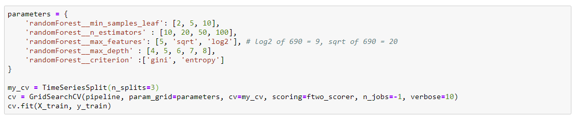
Even though we only started out with only a few technical indicators, the secondary indicator combinations and the use of 20 days of prior history led to having 690 columns. This made the hyperparameter tuning slow and limited more extensive exploration of additional models and hyperparameter combinations due to limitations in local computational resources.
In addition to using the GridSearch, the excellent auto-ML tool TPOT was used for on overnight optimization run. The TPOTClassifier identified a Gaussian Naive Bayes classifier with its default parameters as the best performing model.
Results
Model Evaluation via Backtesting
We focused on finding optimized hyperparameters for random forests as a method to predict profitable trades and used different F-Beta scores as the scoring metric. In total, five optimized models were identified: the initial Random Forest, outputs from three Gridsearches with different betas, and the Gaussian Naive Bayes classifier.
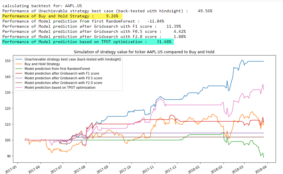
The performance of the models was inspected with several metrics such as confusion matrix, accuracy scores, and the sklearn classification report. However, all these metrics are only indirect indicators of the true quality of the predictions since these metrics don't include any information about the timing of the predicted trade recommendations and the cumulative impact they will have on an investment. The only real way to assess the quality of the predictions is to simulate executing the trades as per the strategy and comparing the financial performance of the different models to the theoretical best case (y_train - trading with perfect hindsight) and to a simple buy-and-hold strategy.
In order to calculate the trade performance, we built a backtesting method that can "replay" the stock prices, act on the trade recommendations, and keep track of the cash position or number of stocks owned, and calculate the value of the holdings/cash over time. The performance at the end of the time period tested was calculated and performance charts were generated to validate the robustness of the models.
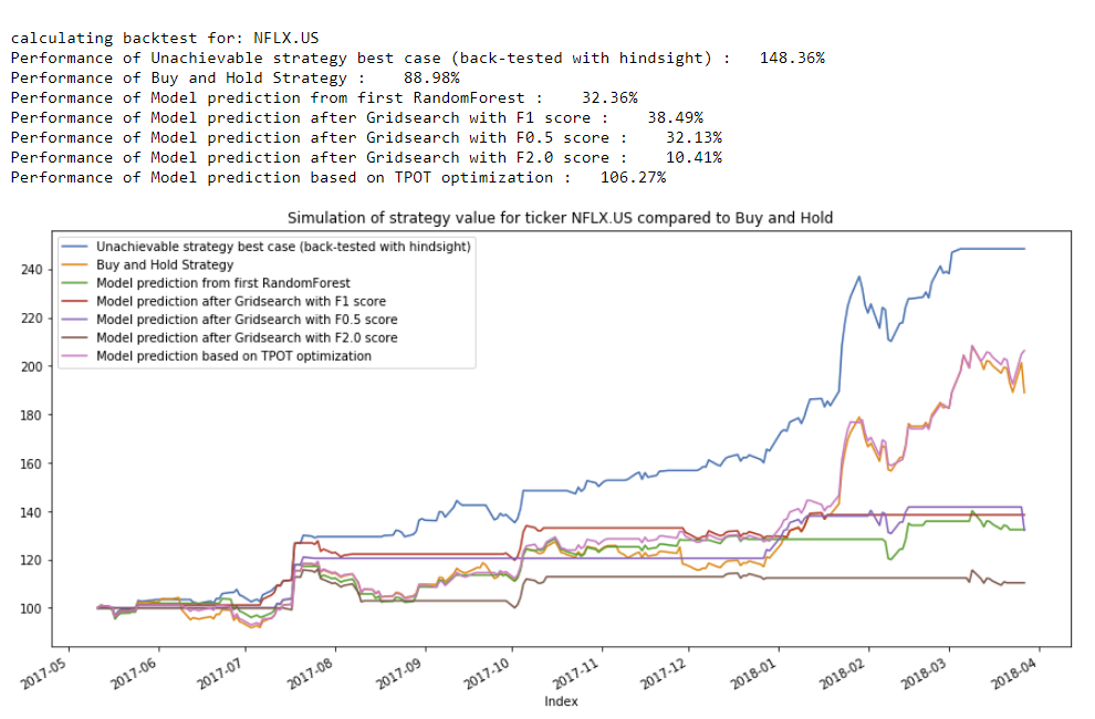
Below is an example of the value (normalized to 100 as starting capital) for trading the stock of Netflix (NFLX) based on trade recommendations from the different models - in this example, the GaussianNB Classifier slightly outperformed the buy-and-hold strategy:
In the next example, we compare the performance of recommendations on trading the stock of Amazon:
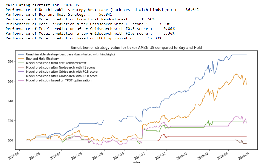
Carefully inspecting these backtests and those for the remaining stock symbols in the test set, the GaussianNB classifier identified by TPOT emerges as the best performer as it was able to outperform the buy-and-hold strategy for several stocks.
Despite the GaussianNB classifier performing the best, the optimized RandomForest classifiers provide us an additional insight when we review the ranked feature importances: the features of type "SMAx to SMAy ratio" consistently appeared very high in the list of important features. This provides cues towards how to continue future iterations of this modeling process and where to focus on feature development.
Overall, the performance of the model predictions is not great and a simple buy-and-hold strategy would have generated better results during the evaluation period. During the modeling process, different scoring metrics were used. The RandomForest classifiers did not appear to clearly perform better for one of the beta parameters over the others. In order to leverage and explore multiple additional model types, TPOT was used to find a better model type.
Improvement Opportunities
This project focused heavily on building out the foundation of preprocessing and backtesting model results. There are now numerous additional avenues for improving prediction capabilities for this problem set. A few are listed here with initial thoughts on why/how they would help:
-
- Using the backtest result as the scorer: instead of optimizing the model training based on F-beta scores or other metrics such as precision, recall, or accuracy, the backtest could be used as a scorer. Optimizing the financial performance of the predictions should significantly improve model performance. However, calculating the backtest in the current implementation is not an efficient vectorized calculation but a loop. The performance of evaluating this custom scorer would likely be very slow leading to much longer model training times.
- Based on the identified feature importances, remove some of the lower ranked features for quicker training due to fewer features. PCA might be used to automate this process but this might be very slow on an individual computer.
- Adding more different stock tickers to the training set: this would allow for better but also much slower training.
- Using a parallelization framework like Dask to improve training speed by using multiple computers for training.
- Adding additional technical indicators as features to extract additional higher-level information from the stock price data.
- Bringing in completely external data such as Twitter sentiment, economic indicators, or even news data on the covered stocks. This would add a whole new dimension of complexity to the modeling process but would likely be very helpful.
- Updating the preprocessing steps to improve performance by vectorizing some of the calculations and using fewer loops.
- Test different trading strategies so see if models can learn other equally profitable strategies better.
Conclusion
We set out to predict profitable trading opportunities. The overall goal was to implement one specific trading strategy: buy a stock the next day when the stock market opens, hold it for another nine days, and sell it. This way, we were able to recast a time series prediction into a classification problem (buy or don't buy).
We obtained a dataset of historical stock prices, calculated the training target (the trade signals), augmented the data with technical indicators (we kept it simple and only used Simple Moving Averages and Relative Strength Index), built higher-order indicators such as crossovers, and reshaped the data such that we could include performance from prior days into our predictions made for day N.
We then trained several models on the dataset to identify optimized model parameters. The model training turned out to be computationally more expensive than initially estimated and limited how much progress we could make on quickly getting to a highly performant model. However, this is not really that surprising since big hedge funds and other investment firms spend significant amounts of resources on developing quantitative trading strategies such as this and even they don't easily find great performing models that instantly create large outperformance over the market performance.
The final challenge in this project was to build a backtesting method to understand the true performance of the model predictions since the standard classification metrics are not very useful to understand the performance of these predictions that act on a time series.
With the preprocessing, model parameter tuning, and backtesting in place, we evaluated the predictive capabilities of 5 different models on a test set and identified a Gaussian Naive Bayes model as the best performer. Finally, we identified several opportunities on what we could improve on this project in future iterations.
The source code for this project can be found at https://github.com/Lindstaedt/Stock-recommendation-with-ML